Ciclop: building a laser 3D scanner from a kit

Last month at Quark our table held three machines: the submarine, the wall-drawing plotter, and a 3D scanner built mostly out of 3D printed parts. This post is about the scanner, the geometry that makes it work, and the part the kit documentation skips, which is everything after assembly.

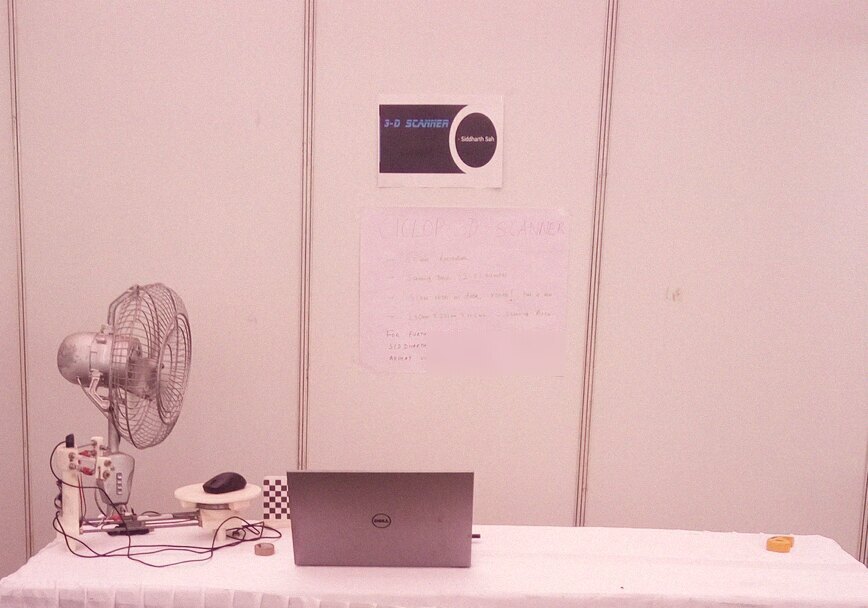
The handwritten poster claims 0.5 mm resolution, two to three minutes per scan, a 250 x 250 x 205 mm scanning volume, and scanning in the dark. All of those held up with a festival crowd poking at the machine. The 0.5 mm number falls straight out of the geometry, as below, and the last claim is my favorite, for reasons further down.

Why build a scanner

The Aerodynamics Club printer will make any part you can model. The bottleneck is the modeling, because most of what you want to copy already exists as an object on your desk. A scanner closes that gap: digitize the thing, edit the mesh, print the edit.

We picked Ciclop, BQ’s open-source laser scanner (files released under Creative Commons), over Atlas and FabScan, after reading a lot of scanner documentation. FabScan’s bachelor thesis is good reading. The design is printed parts and M8 threaded rod, an Arduino UNO under a ZUM shield, one stepper on a turntable, a Logitech webcam, and two line lasers that cost one hundred rupees.

How laser triangulation works

The principle is triangulation. A line laser projects a vertical plane of light. The webcam watches from a known angle. Wherever the line lands on the object, its sideways displacement in the image encodes depth, one slice per exposure. The turntable rotates the object through a known step angle between slices, and because the rotation is commanded, registration comes free. Every slice already knows its angle, so no alignment algorithm runs.

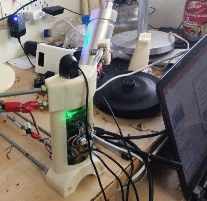
The capture software is Horus, BQ’s open-source companion. It drives the board, streams the webcam, and assembles the point cloud live on screen. Watching the first cloud take the shape of a shampoo bottle was a good moment.

The math

The camera is a pinhole model. A 3D point in front of the camera projects to a pixel through the intrinsic matrix K, which holds the focal length in pixels and the image centre, plus a couple of lens distortion coefficients so straight edges don’t bow near the frame edges. OpenCV estimates all of it from a dozen photos of the checkerboard at different tilts. That’s what the checkerboard is for.

A laser plane is a plane in the same frame, n · X = d. To find it, you photograph the stripe falling across the checkerboard at several tilts. The board’s pose in each photo is known from the calibration, so every stripe pixel maps to a 3D point on the board, and a least-squares plane fit through those points gives n and d. Our fit was good to about 0.15 mm, which set the floor for everything downstream.

Scanning is then one formula per pixel. A stripe pixel (u, v) becomes a ray r = K⁻¹ [u, v, 1]ᵀ. The ray meets the laser plane at

X = (d / (n · r)) * r

one point in the camera frame. Rotating X by the turntable’s commanded angle puts it into the object frame, and that’s one point in the cloud. Eight hundred slices, a few hundred stripe rows each, and the cloud is a few hundred thousand points.

Depth resolution comes from the geometry. A one-pixel shift of the stripe corresponds to a depth change of about dz = z² / (f b), where z is the distance to the object, f the focal length in pixels, and b the distance between laser and camera. Our webcam has f ≈ 800 px, the laser sits 150 mm from the camera, and the object sits 250 mm out, so dz ≈ 250² / (800 × 150) ≈ 0.5 mm per pixel. That’s the poster’s number. The subpixel centroid could in theory do better, but calibration error and bearing wobble are larger.

The turntable is a 200-step motor at 1/16 microstepping, 3,200 microsteps per turn. At 800 slices per revolution that’s 0.45° per slice, an arc of about 0.8 mm at the edge of the volume, so slices are spaced a little coarser than the depth resolution. Finer steps mean longer scans, and past a point they add no resolution. That’s where the poster’s two-to-three-minute range comes from.

Getting usable scans

Assembly is an afternoon. Getting scans worth keeping took months, and that was most of the work.

The webcam is the first problem. A stock Logitech runs autoexposure and autofocus, and both are bad for laser detection. The exposure changes with the room, the laser line blooms and thins between frames, and the segmentation threshold that worked at noon fails at six. Locking exposure, focus, and white balance manually was the single biggest improvement in scan quality we found. On Linux that’s three v4l2-ctl calls before every session: manual exposure at a fixed absolute value, autofocus off with the focus set for the turntable distance, and auto white balance off. No assembly guide mentions it.

Turning the lights off is the second. Horus segments the laser by thresholding what the camera sees, and the easiest way to help it is to remove everything else red from the frame. In a dark room the laser is the only red thing in the frame and background subtraction becomes trivial. The poster’s “scanning in the dark” claim is really a description of the scanner working at its best.

Surfaces are the third. A red line laser fails on shiny, dark, and translucent objects. Specular surfaces throw the line somewhere else, dark ones absorb it, and translucent ones glow from inside. The community fix is a light dusting of talcum powder, so a talc tin lived next to the scanner and everything difficult got scanned in matte white.

The mechanics show up in the data. A cheap turntable bearing has wobble, and the wobble shows up as a ripple around every scan at exactly the rotation frequency, about 0.3 mm on ours, the same order as the depth resolution. We learned to read point clouds the way we had learned to read failed prints.

We also ran comparison experiments the kit doesn’t ask for. One laser or two is a real question. The second laser halves occlusion shadows and doubles the calibration burden, and a slightly misaligned second plane ghosts every surface twice. A plane error of 0.3° at 250 mm standoff puts the two surfaces 250 × tan 0.3° = 1.3 mm apart, which is what the double wall in our jar scan measures. The archive has a dibba_singlelaser.ply from the night we settled it. We tried photogrammetry on the side. The laser won on repeatability at this budget.

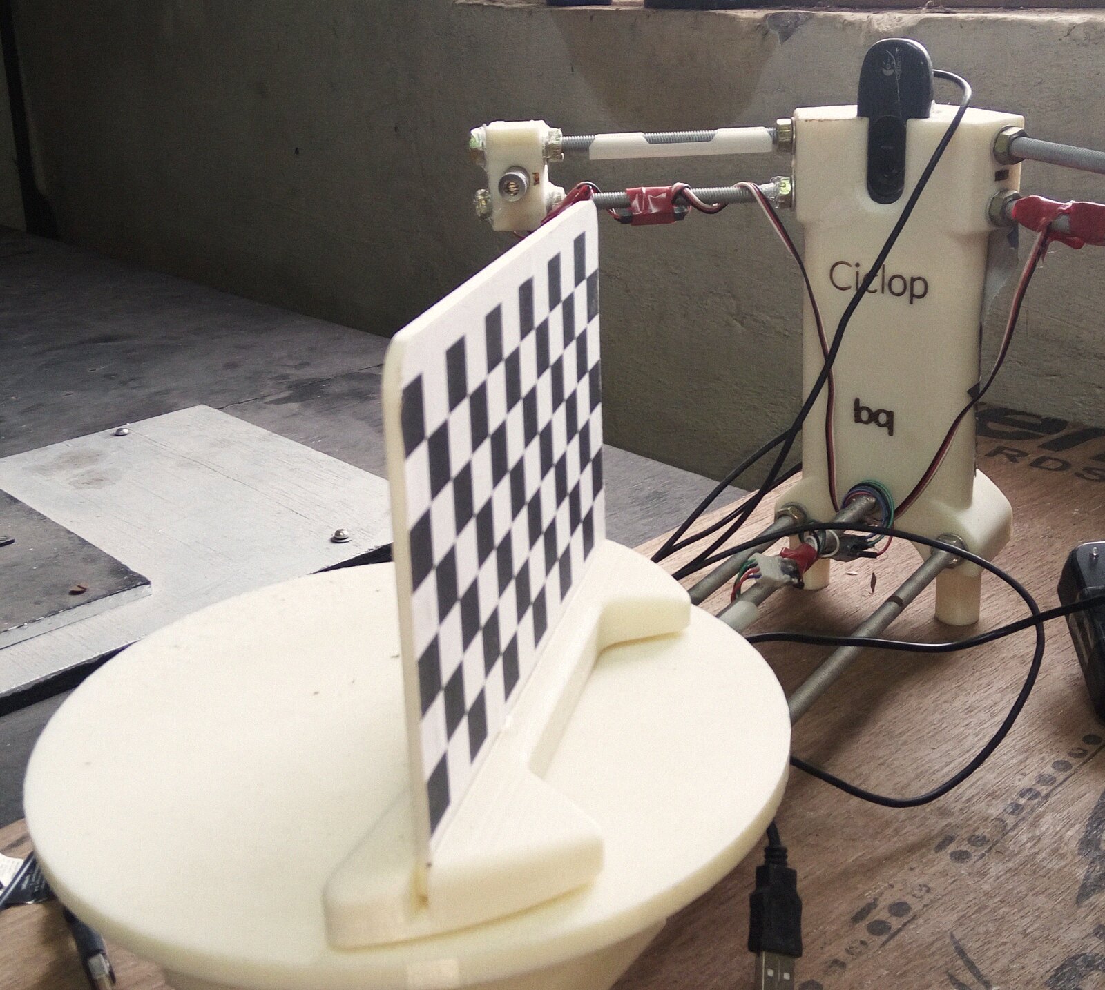
All of this sits on calibration. The checkerboard calibrates the camera intrinsics, then the laser planes, then the turntable axis. The printed structure is really a jig for holding those three calibrations steady. Bump a laser mount and the hardware is fine while every scan is garbage.

How Horus processes a scan

Horus is a Python desktop application built on OpenCV. It runs the machine over a serial line, using G-code-style commands to switch each laser and step the turntable one fixed angle per slice. For every slice the capture loop grabs a frame with the laser on and one with it off, subtracts the pair to remove the room, computes a red-dominance ratio R / (G + B + 1) and thresholds it, which holds up under warm room light better than thresholding the red channel alone, and collapses the stripe to a per-row weighted centroid. That places the line’s center between pixels, at a fraction of a pixel’s width.

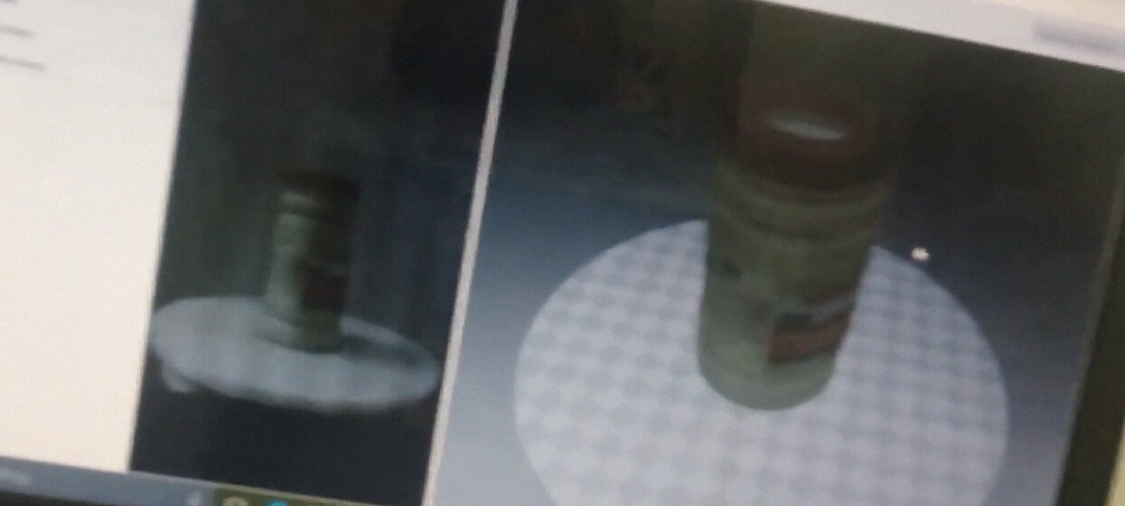
Every centroid then goes through the ray-plane intersection above. The whole scanner is three coordinate transforms run eight hundred times per revolution.

Our additions live around the edges of that loop. A camera script forces exposure, focus, and white balance to fixed values before every session, because segmentation constants are useless while the webcam keeps changing the image. Threshold presets per material class (matte, dark, and shiny-after-talc) saved retuning from scratch every night. And cleanup moved into meshlabserver, MeshLab’s headless mode, so outlier removal, normal estimation, and Poisson reconstruction ran with identical parameters on every cloud. Two scans of the same object stayed comparable.

Point cloud to STL

Horus exports .ply point clouds, and clouds aren’t printable. The pipeline runs through MeshLab: statistical outlier removal for the stray points the threshold let through, normal estimation, Poisson surface reconstruction to close the surface, then export to STL for the printer. Poisson takes a depth setting, and 9 gives cells around 0.5 mm on this volume, matched to the scanner. One step finer quadruples the mesh and only reconstructs the noise. The file names in the scans folder show how it went, from test_toi and first_deo (a deodorant can) to the night one file got saved as insane.ply, which is what you name a scan when it finally works.

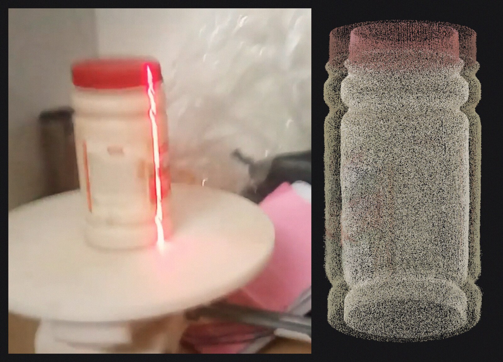
That file is the jar. 891,105 colored points, the lid still red, and a faint double shell where the second laser disagreed with the first by a hair. That’s a calibration error you can see in the data.

The bill for the whole machine came to about ₹14,000. The two lasers cost a hundred rupees, and the printed structure cost more than all the electronics combined. The parts came off the same class of machine the scanner now feeds, so the loop closes in both directions. The printer made the scanner, and the scanner makes files for the printer. Being able to copy an object off my desk, edit it on the way through, and print it, for less than a textbook, still feels a bit unreal.

What we learned

1. Lock the camera before trusting the math. Every segmentation constant assumes yesterday’s exposure, and an autoexposure webcam changes that every frame. Three v4l2-ctl calls before each session fixed more scans than any other change.
2. You can tell the cause from the shape of the defect. A double wall 1.3 mm wide is a second laser plane off by 0.3°. Ripple at once per revolution is the bearing. Fuzz everywhere is the threshold.
3. Use the same parameters for every scan. With one meshlabserver script on every cloud, two scans of one object differ only by the scanner.
4. The coarsest step in the pipeline sets the resolution. Our 0.5 mm came from z²/(f b) at the standoff distance. Polishing the subpixel centroid past that did nothing, and the 0.79 mm slice spacing at the volume’s edge was coarser still.
5. A festival crowd is a free stress test. Two days of strangers spinning the turntable by hand found weaknesses two months of careful sessions never touched.
6. The STL files are open source. The part a repository can’t hold is the practical knowledge: which talc on which surface, which threshold for which evening light. Write that down too.