DeepSafe: running 21 deepfake detectors behind one API

The deepfake detection literature has a distribution problem. The models exist, the papers are good, and almost nobody outside a lab can run any of it. Every research repo ships its own broken environment, its own weight files on a link that dies within a year, and its own Python version requirement. Meanwhile the fakes ship as consumer apps. DeepSafe is my attempt to fix that: take the best open detectors, make them run in one place, and put a single URL in front of them. The code is open source. This post is about how the engineering works, down to the import system and the calibration math.

One process for all 21 models

The current build runs twenty-one detection services across three modalities: seven image detectors, three audio detectors, and nine video pipelines, two of which are image detectors run across frames. They load into a single GPU process at startup and answer as in-process function calls.

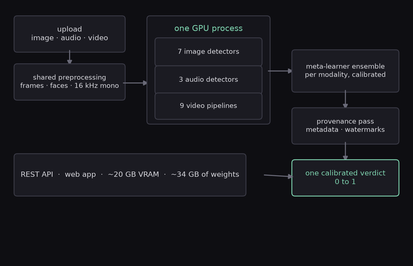
The first architecture was the obvious one, a container per detector, and it was a mistake. Every process that touches the GPU creates its own CUDA context, and a context costs 300 to 500 MB of VRAM before a single weight is loaded, plus a resident copy of PyTorch and its kernels in host memory. Twenty-one of those is 8 GB of VRAM spent on bookkeeping, and the fragmentation across contexts means no scheduler can pack the models in. Collapsing everything into one process traded all of that for a single context and function-call latency between gateway and model.

Getting research code from that many authors into one process is its own project, because every research repo ships a module named models, a module named utils, and a module named data, and Python’s import system allows exactly one of each name in sys.modules. The fix is namespace isolation. Each detector’s code is imported under its own prefix so the duplicate utils modules never meet.

imported = namespaced_import_multi(
    code_path=detector_dir,
    namespace="_ds_detector_07",
    import_specs=[{"module": "models.net", "attr": "Detector"}],
)

Under the hood that function loads the detector directory as a package under its own name using importlib, registers it in sys.modules under the prefix, and rewrites the detector’s own from utils import x lines to from _ds_detector_07.utils import x before executing them, so every import inside the vendored code resolves inside its own namespace. The prefix trick costs forty lines. The one thing it can’t isolate is a compiled C extension with a hardcoded module name, and two detectors needed a small shim for that.

Every wrapper subclasses one BasePredictor, so a detector is a directory, a weights file, and a class with a predict method, and adding one never touches another. All the model code is vendored into the repo, and roughly 34 GB of weights live in one storage bucket, so setup is one command and the machine never touches the internet at inference time.

The other shared plumbing is preprocessing, because the expensive work is identical across detectors and should run once. Video gets decoded once into eight uniformly sampled frames plus a dense track capped at ninety. Face detection runs once with SCRFD, which benchmarks several times faster than the MTCNN most research repos default to, and every detector that needs faces gets the same crops, the detected box with some margin, aligned on the eyes and mouth, resized to each model’s input. Audio gets resampled once to 16 kHz mono and padded or trimmed to 64,600 samples, the 4.04-second window the ASVspoof lineage standardized.

Concurrency, VRAM, and failure handling

The fan-out uses a plain Python thread pool. That works because inference spends its time inside CUDA kernels, and PyTorch releases the interpreter lock before launching them. The GIL only hurts workloads that live in Python, and after shared preprocessing these don’t. Each worker thread gets its own CUDA stream, so kernels from different detectors can overlap on the device. The payoff is latency. A request costs the slowest detector’s forward pass, where sequential dispatch would cost the sum of all of them.

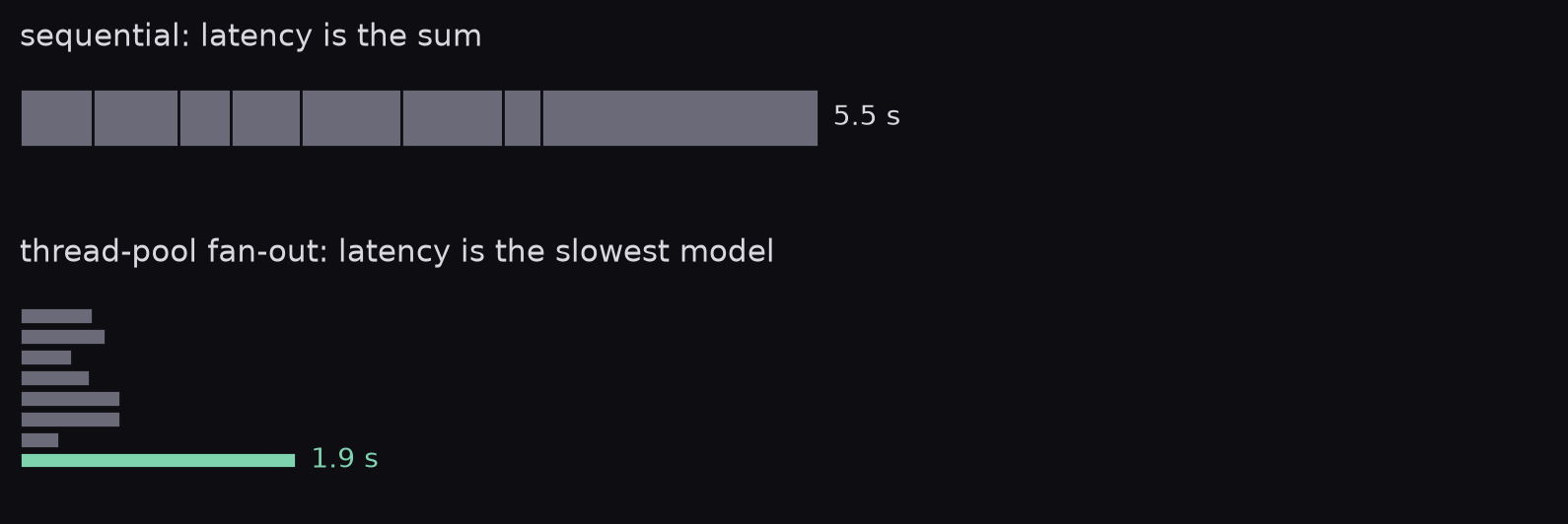
Each wrapper call carries its own timeout so one hung forward pass can’t block the verdict. The timeout is implemented with concurrent.futures.wait, and it has a limit worth knowing: you can’t cancel a running CUDA kernel from Python. When a detector times out, its future is abandoned, its vote is imputed as below, and the thread returns to the pool whenever the kernel finishes. A detector that times out three times in a row is marked unhealthy and skipped until the next health sweep reloads it.

Every model stays resident from startup, because cold-loading a multi-gigabyte checkpoint costs seconds while a resident model answers in tens of milliseconds, and users won’t wait for the first kind. Half-precision residency is what makes the memory work out, near 20 GB for the whole set. FP16 tops out around 65,000, and two models overflow it in their last layers, so those two run at full precision under a per-model flag and the rest use autocast. One shared PyTorch allocator manages the pool. With containers there would be twenty-one of them fragmenting twenty-one arenas.

The downside of one process is that one bad model can take everything down, and that’s the strongest argument for the container design. The mitigations are simple. Every wrapper call is fenced by its own exception boundary, a model that starts failing gets marked unhealthy and its vote dropped, and the ensemble imputes the missing feature at that model’s training-set mean, so the platform returns a degraded verdict with a flag on it and never a 500. The meta-learners were trained with random feature masking, ten percent of votes dropped per training row, so a missing vote at inference time looks like something they’ve seen. The health endpoint exists because the degraded state is normal. With this many models, something is usually broken.

Every verdict can be checked after the fact. The response carries each model’s probability and latency alongside the final score, the per-model endpoints let you re-run the one detector whose vote looks strange, and the ensemble artifacts (meta-learner, scaler, and calibrator) are versioned files, so any verdict can be replayed against the exact model set that produced it.

The ensemble

Averaging the probabilities would assume the detectors are equally good and equally independent, and they’re neither. The families fail differently. The frequency-domain detectors take a Fourier transform of the image and look for the periodic peaks that a generator’s upsampling layers leave in the high frequencies. They’re strong on GAN output and weak on anything re-encoded through a lossy codec. The backbone classifiers are EfficientNet and Xception variants fine-tuned on face crops, and they generalize best. The reconstruction detectors run a face through an autoencoder trained on real faces and score how badly it reconstructs, since a generated face doesn’t look like the faces the autoencoder learned. One video detector specializes in mouths, checking whether the lip motion matches the audio track, because lip sync is still the weak point of video fakes. The audio detectors work on spectrogram-like features and on raw waveforms.

So the aggregation layer is itself a trained model: a separate ensemble meta-learner per modality, gradient boosting for images and video and a random forest for audio, each taking the per-model probabilities as features. The meta-learner has to train on votes the base detectors produced for files they never trained on, or it learns to trust whichever model memorized the training set. So the votes come from five-fold out-of-fold predictions over the held-out pool of about 15,500 labeled files (1,465 effective samples for image, 3,346 for audio across dozens of languages, 987 for video).

The last step is Platt scaling, a logistic fit on the meta-learner’s raw score, so the final number behaves like a probability. Calibration is checked with expected calibration error, which bins predictions by confidence and averages the gap between stated confidence and actual accuracy. A verdict that says 0.9 should be wrong about one time in ten, and the image ensemble’s ECE of 0.0096 means it is.

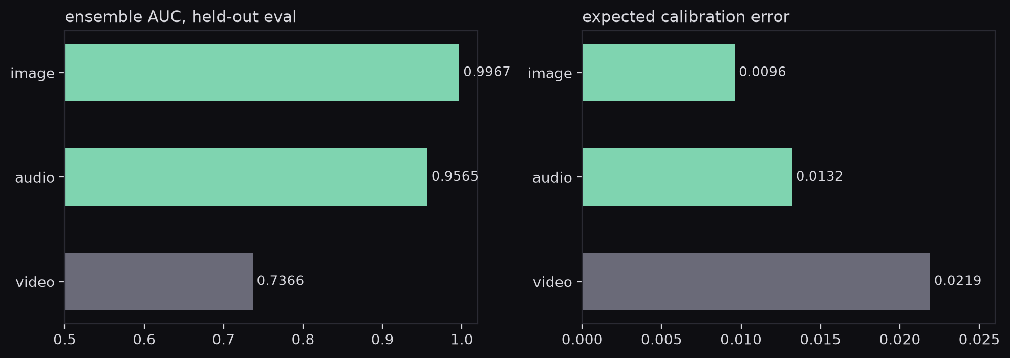
The image ensemble reaches 0.9967 AUC on the held-out evaluation, audio reaches 0.9565, and video manages 0.7366. I publish all three numbers because the third one is the one that matters. Video deepfakes are still the hard problem, and any product that claims otherwise is overstating it.

Building the ensemble was mostly removing detectors that didn’t perform. One audio detector graded at 0.199 AUC, worse than a coin flip and anti-correlated with the truth, and it survived a week longer than it should have because its README was excellent. Another scored 0.367 on speech because it was built for AI-generated music, which its abstract mentions once. Every model has to justify its place on the evaluation set, whatever the paper says.

Provenance checks

Classifier scores are one kind of evidence. The other kind is written into the file: C2PA content credentials, generator metadata, and the invisible watermarks some generation tools embed in their output. A C2PA check is three steps. Find the manifest embedded in the file, recompute the hashes it lists (including the hash of the image bytes it claims to describe) and compare, then verify the signature over the manifest against the signer’s certificate. A manifest that says “created by a generative model” and verifies settles the question. A manifest that fails its hash is evidence of editing after signing. No manifest at all means nothing, because almost nothing carries one yet.

DeepSafe runs these provenance checks as a second stage, and the merge is asymmetric. A watermark is strong evidence of generation and a missing watermark means nothing, so provenance can push a score toward fake and never toward real.

boost = (max_provenance - 0.5) * weight  # 0.20 strong signal, 0.05 weak
final = score + boost * (1.0 - score)    # moves toward 1, never past it

A moderate signal nudges, a definitive signal overrides, and the shape of the formula guarantees the classifier’s score is the floor.

The API

Detection is useless behind a conda environment, so the models sit behind a FastAPI inference server with a gateway in front for auth and rate limiting. POST /v1/detect takes a multipart file and returns one calibrated verdict. Every model also exposes its own endpoint, so a single detector can be queried when its vote looks strange, and GET /health reports per-model status. The web app is simple: drag a file in, or paste a URL, and read a number.

The training data comes from the public benchmarks the field grew up on, FaceForensics++ and the Deepfake Detection Challenge among them, and the generators keep changing. GANs made faces, and their upsampling artifacts are what half the image detectors were built to see. This summer’s diffusion models make everything, and they leave different artifacts. The detectors will need retraining as the generators change, and that won’t stop.

What I learned

1. Evaluate every detector yourself before it touches the ensemble. Two published models scored below a coin flip on my test set, and one of them was anti-correlated enough to be useful upside down.
2. The weakest modality sets what the product can promise. Image AUC of 0.9967 is a nice line until a video arrives, so the video number, 0.7366, is the one that belongs in every conversation about what the tool can do.
3. Calibrate the output. An uncalibrated 0.93 means nothing to the person deciding whether to trust a video of their CEO. Platt scaling is twenty lines, and ECE tells you whether it worked.
4. Vendor the code, mirror the weights. Half the detectors I evaluated had a dead weight link within a year of publication.
5. Namespace isolation beats containers for a model zoo. One process holding all the models pays for a single CUDA context where containers would pay for twenty-one, and the import prefix trick costs forty lines.
6. Train the meta-learner on out-of-fold votes and with votes randomly masked. Without the first it learns to trust the model that memorized the training set. Without the second, a single unhealthy detector produces a verdict the ensemble has never seen.
7. Provenance beats inference when both are present. A C2PA check is cheap and definitive, so run it first.
8. Design the degraded mode before the demo. With this many models one is always broken, so the missing-vote path (imputation plus a flag in the JSON) is a first-class feature.